Guide to HeyVL
For a short introduction to running Caesar and interpreting a verification result, start with First Example: Expected Runtime. This guide explains HeyVL in more detail, using a lossy list traversal to introduce user-defined types and functions, quantitative specifications, and loop invariants. It then explains the verification statements used to encode proofs in HeyVL.
Contents of This Guide
What Are HeyVL and Caesar?
Architecture
Architecture of Caesar
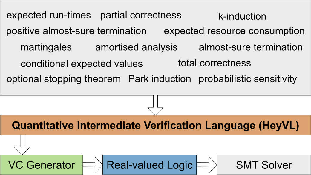
On the right, you can see the architecture of Caesar. Caesar is designed as a deductive verification infrastructure for probabilistic programs.
At the core is HeyVL, our intermediate verification language (IVL).
An IVL is used to encode a wide range of verification problems and verification techniques into a common language.
In contrast to normal programming languages, IVLs can feature statements such as assert and assume.
Intuitively, assert checks a condition and fails if it's not true.
assume lets us make a logical assumption at arbitrary points in the program.
These can be used to encode proofs and proof rules into the IVL.
HeyVL is a quantitative IVL, meaning that its verification statements (assert, assume, havoc...) do not only reason about Boolean statements (x = 3), but rather about quantities such as expected values ([x = 3] * 0.5).
The verification condition generator (VC generator) converts a HeyVL program to a formula in our quantitative logic HeyLo.
This formula expresses the proof obligations of the HeyVL program.
For example, assume [x = 3]; assert 0.5 is converted to the HeyLo formula [x = 3] → 0.5.
We will explain what this means later in this guide (see the section on verification statements).
At the end, Caesar converts the HeyLo formula into a problem for an SMT solver; currently we use Z3.
This allows us to check whether a program verifies for all possible inputs.
If verification fails, then the SMT solver can often return a counter-example, i.e. an input to the program so that the program does not verify.
Caesar supports a number of proof rules out of the box (see proof rules documentation).
For example, reasoning about while loops or recursion is done through proof rules.
By adding an annotation such as @invariant to a while loop, you instruct Caesar to use the Park induction proof rule.
However, this will internally desugar into normal HeyVL code which means these proof rules are not magic built-ins, but just a convenience in Caesar.
Thus, you can add your own proof rules with Caesar by encoding them in HeyVL.
That is the advantage of using an intermediate verification language such as HeyVL.
Our OOPSLA '23 paper (PDF) gives the formal foundations of HeyVL and explains how to prove that its encodings represent the intended verification problems. The CAV 2026 tool paper describes Caesar's architecture and current capabilities.
Features
So, what can we do with HeyVL and Caesar right now? Here's an incomplete list of features:
- Prove correctness and find bugs in probabilistic programs.
- We have verified properties like lower and upper bounds on expected values, such as expected values on termination, expected runtimes, expected resource consumption, termination probabilities, and more.
- Using proof rules like Park induction, k-induction, rules for positive almost-sure and almost-sure termination, or the optional stopping theorem.
- Use HeyVL, a quantitative intermediate verification language that
- has generalized quantitative verification statements
assume,assert,havoc, and nondeterministic choice, - features dual co-versions of verification statements to reason about upper bounds of expected values (the non-
costatements are used to reason about lower bounds), - and through these allows you to encode new proof rules and use Caesar as a verifier for them.
- has generalized quantitative verification statements
- Use SMT solvers to reason symbolically about infinite-state probabilistic systems, unbounded loops, and recursion.
- Compositionally reason about programs, building bigger verified programs out of smaller verified parts using procedures.
- Define your own data types and define new functions in HeyVL, with support for uninterpreted definitions, i.e. those defined by logical axioms and thus may not even have an executable definition.
- Formally correct reasoning with theoretical guarantees. We do not use sampling algorithms such as MCMC, but instead use logical reasoning about programs.
Example: Lossy List Traversal
The geometric loop in the first example uses a Boolean variable and a constant bound on expected runtime. Here, we introduce a list type and prove a bound on the probability that a traversal succeeds, expressed as a function of the list's length. The full example can be found below.
The Probabilistic Program Itself
Let us start with the probabilistic program itself, without any HeyVL annotations.
lossy_list is a procedure that takes an input init_l of type List and returns an output list l.
List is a user-defined type which we define below.
proc lossy_list(init_l: List) -> (l: List)
{
    l = init_l
    while len(l) > 0 {
        var prob_choice: Bool = flip(0.5)
        if prob_choice {
            l = pop(l)
        } else {
            assert [false]
        }
    }
}
The program is supposed to model a list traversal with a (rather alarming) 50% probability of memory faults during the traversal. For this guide, we want to prove a lower bound to the probability of a successful traversal.
What Does the Program Do?
-
We initialize the output
lto the input. Note that it's forbidden in HeyVL to modify input variables. -
The main part of the code is the
whileloop. It runs as long as the length oflis nonzero.-
In the loop body, we have our probabilistic statement: The
flip(0.5)expression does a coin flip and returnstrueorfalse, each with probability0.5. The result is saved in a newly declared variableprob_choiceusing thevarstatement. When we declare a new variable in HeyVL, we always need to specify the type. -
If the coin flip resulted in
true, then we remove the first element of the top of the list usingpop. The resulting list has a length that's one smaller than before. -
If the coin flip resulted in
false, then we simulate a memory fault usingassert [false]. - Deductive verification requires a proof-rule annotation for this loop. We add an invariant in the section on specifications.
-
-
HeyVL does not have
returnstatements. Every value to be returned by the procedure must be declared as an output variable in the procedure declaration. Here, the output variablelis automatically returned.
There is more detailed documentation on HeyVL's procedures and statements.
What Do We Want to Verify?
With Caesar, various properties of this program can be verified:
- In this guide, we'll only verify that the probability of a successful run without crashing is at least
0.5^len(init_l). - We could verify probabilities of crashing at specific list lengths.
- We could verify expected values of list lengths at crash time.
- For the above, we can verify either lower or upper bounds.
- The program is certainly terminating, i.e. each execution will always terminate in a finite number of steps.
- There are programs that only terminate with probability one, but may have a zero probability of not terminating. We call these programs almost-surely terminating (AST for short).
- There are programs which terminate with probability one, but do not have a finite expected runtime. Such programs are almost-surely terminating, but not positively almost-surely terminating (PAST for short).
- ... and many more.
User-Defined Datatypes and Functions
Our probabilistic program above is incomplete: it's still missing a specification and a loop invariant annotation.
In addition, the List type and the exp function need to be defined.
They are not built-in into HeyVL, but must be axiomatized using user-defined domains and functions.
How this works is that domains and functions are defined uninterpreted, which means that they do not necessarily need to have a complete executable definition associated with them. Domains are simply new types which functions can map from and into. Functions simply have input and output types.
Then, axioms define the knowledge that Caesar (and the underlying SMT solver) will receive about these uninterpreted domains and functions. For the purpose of verification, we check all possible definitions which satisfy these axioms and ignore those that do not satisfy them.
The List Type
Let's declare our list type, using the built-in UInt type for nonnegative integers.
domain List {
    func len(l: List): UInt
    func pop(l: List): List

    axiom list_pop forall l: List. len(pop(l)) == len(l) - 1
}
You will notice that we do not declare what a list consists or what size the data type should have.
We simply declare a domain List and have two uninterpreted functions len and pop operating on this type.
They also don't have definitions, but only the axiom list_pop that says the length will decrease by one if we run pop on a list l.
These uninterpreted definitions are part of the magic of deductive verification using SMT solving that Caesar does.
We can simply define new types and functions logically via a (possibly partial) specification and verify with those.
This makes Caesar very extensible: new definitions do not need to be baked into Caesar itself, but can be defined by the user.
This makes axioms also extremely dangerous. Consider axiom my_wrong_axiom false.
Because false is never true for any interpretation, verification with this axiom will always succeed!
The Exponential Function
Remember that we want to prove a lower bound of 0.5^len(init_l) for the probability of a run without crashing.
Exponential functions are also not included in Caesar, but it can also be easily added.
domain Exponentials {
    func exp(base: UReal, exponent: UInt): UReal

    axiom exp_base forall base: UReal. exp(base, 0) == 1
    axiom exp_step forall base: UReal, exponent: UInt. exp(base, exponent + 1) == base * exp(base, exponent)
}
We declare a domain Exponentials.
The new type Exponentials is not used, but all function definitions and axioms need a surrounding domain.
The function exp takes a base and an exponent of type UReal and UInt, respectively.
See the number types docs for more information.
There are two axioms for exp.
The first, exp_base specifies that exp(base, 0) == 1 holds for all base values.
The second, exp_step specifies the successive cases, exp(base, exponent + 1) == base * exp(base, exponent).
You might wonder why we specify the exponential function in this inductive way and not via the many other definitions of the exponential function that Wikipedia provides. After all, we are not restricted to inductively computable definitions and can use any logical specification we want, right? The answer here is that those two axioms are precisely the ones needed to prove our specific property using our chosen proof rule of Park induction. We'll see this below. In general, what axioms you need to provide for verification is often specific to the verification task at hand.
Refer to the documentation on domains and functions for more information.
Specifications and Invariants
Now that we have provided all necessary definitions for the program, let us write the specification.
Remember that we want to verify that the probability of a successful run without crashing is at least exp(0.5, len(init_l)).
How do we specify such a property in HeyVL?
HeyVL uses expectation-based reasoning, which is a kind of deductive reasoning that talks about expected values of random variables. We describe the full theoretical details in our OOPSLA '23 publication. For now though, we'll provide some intuition.
Specifications
We extend our lossy_list declaration as follows with a pre and a post attribute:
proc lossy_list(init_l: List) -> (l: List)
    pre [len(init_l) == 1] * 0.5
    post [true]
{ ... }
What does this mean?
Expectation-based reasoning always works backwards through the program.
Accordingly, we start our interpretation with the post.
The procedure having the post [true] means that we are ultimately interested in reasoning about the expected value of [true] at termination.
The Iverson bracket notation [b] maps a Boolean expression b to 1 if b evaluates to true and to 0 otherwise.
Therefore, [true] is equivalent to 1.
It follows that post [true] means we are interested simply in the probability of successful termination.
The pre [len(init_l) == 1] * 0.5 is a bit more interesting.
It results in a proof obligation for Caesar: the verifier now needs to show that the pre is always a lower bound to the expected value of the post.
The pre evaluates to 0.5 in case the length of the list is exactly one and to zero otherwise.
Since the pre is checked as a lower bound (and expected values are nonnegative in HeyVL), Caesar in effect only checks that 0.5 is a lower bound for inputs with list length equal to one.
Of course, we can also change the pre so that Caesar has to check infinitely many inputs, e.g. by changing the pre to [len(init_l) != 1] * exp(0.5, len(init_l)).
Thanks to the magic of deductive reasoning and SMT solvers, this will also work instantly.
Invariants and Other Proof Rules
Verification of programs with loops might require reasoning about an unbounded, possibly infinite number of loop iterations. In deductive verification, we reduce reasoning of programs with loops to HeyVL programs without loops. This is done using various proof rules.
In the non-probabilistic setting, the most famous one is the proof rule from Hoare logic (for partial correctness) which says that if we have an invariant for a loop, i.e. a formula that holds before the loop and is maintained during the loop body's execution, then we may conclude that the invariant holds after the loop as well. There is a direct correspondence to this rule in the probabilistic setting. We call this rule Park induction.
To prove the desired pre being a lower bound on the expected value, we need find a probabilistic invariant I, i.e. an expression that computes an expected value for every program state, such that
- If the loop condition is true, then
Imust be a lower bound to the expected value ofIitself at the end of each single loop iteration, - If the loop condition is false, then
Imust be a lower bound to the post (in this case it's[true] = 1).
Note: There is a more formal description on the documentation page for the Park induction proof rule.
This proof rule corresponds to the general proof method of mathematical induction. The base case is (2) when the loop condition is false and the inductive case is (1) when the loop condition is true, where we only reason about a single loop iteration.
So what is a valid invariant for our program?
It turns out that exp(0.5, len(l)) is a valid invariant:
- If the loop condition is true, then the expected value of
exp(0.5, len(l))at the end of the loop iteration is exactlyI! Here's the calculation:0.5 * exp(0.5, len(pop(l))) + 0.5 * 0= 0.5 * exp(0.5, len(pop(l))) (simplify)= 0.5 * exp(0.5, len(l)-1) (list_pop axiom)= exp(0.5, len(l)) (exp_step axiom) - If the loop condition is false, then
Iisexp(0.5, 0)which is equivalent to1by theexp_baseaxiom.
Caesar has built-in support for Park induction with the @invariant annotation for loops.
We add it on top of a loop statement:
@invariant(exp(0.5, len(l)))
while len(l) > 0 { ... }
This is all we needed to do before we can verify this program. Before we do so, a warning.
HeyVL is an intermediate verification language and proof rules like Park induction must only be applied where it is sound with respect to the language semantics that we are considering.
In this case, by using Park induction in a proc, we implicitly assumed greatest fixed point semantics on unbounded non-negative expected values for the loop.
It assigns an infinite expected value to nonterminating executions.
Then, Park induction is sound for lower bound reasoning only.
A more common choice is least fixed point semantics for loops, which assigns zero to nonterminating executions. There, Park induction is sound only for upper bound reasoning (see below).
Refer to the proof rules documentation for more information on soundness of proof rules.
Running the Complete Example
Save the complete program below as lossy_list.heyvl.
domain Exponentials {
    func exp(base: UReal, exponent: UInt): UReal

    axiom exp_base forall base: UReal. exp(base, 0) == 1
    axiom exp_step forall base: UReal, exponent: UInt. exp(base, exponent + 1) == base * exp(base, exponent)
}

domain List {
    func len(l: List): UInt
    func pop(l: List): List

    axiom list_pop forall l: List. len(pop(l)) == len(l) - 1
}

proc lossy_list(init_l: List) -> (l: List)
    pre [len(init_l) == 1] * 0.5
    post [true]
{
    l = init_l
    @invariant(exp(0.5, len(l)))
    while len(l) > 0 {
        var prob_choice: Bool = flip(0.5)
        if prob_choice {
            l = pop(l)
        } else {
            assert [false]
        }
    }
}
Open the file in VS Code and save it to verify with the Caesar extension, or run:
caesar verify lossy_list.heyvl
Reasoning About Upper Bounds (Coprocedures)
In this example, we are reasoning about lower bounds of expected values. In classical non-probabilistic deductive verification, reasoning about lower bounds of truth values is the default and sufficient for most tasks (the recent interest in incorrectness logics being a trend to the opposite). In probabilistic, expectation-based reasoning though, it is just as natural to reason about upper bounds of expected values as about lower bounds. For example, we'd like to prove an upper bound to the probability of a crash. This is not simply the opposite probability to the probability of a successful run when we also distinguish nontermination from crashes (we do!).
HeyVL supports reasoning about upper bounds as well, via its coprocs.
A coproc is just like a proc, but the pre annotation is interpreted differently.
Instead of noting a lower bound on the expected value of the post, it now denotes an upper bound of the post.
The co prefix indicates that the declaration is dual (in a mathematical sense) to the proc one.
HeyVL also has dual co-versions of its verification statements, which will be introduced later.
Consider the following coproc example (with the domain declarations from above omitted):
coproc lossy_list_up(init_l: List) -> (l: List)
    pre 0
    post len(l)
{
    l = init_l
    @invariant(0)
    while len(l) > 0 {
        var prob_choice: Bool = flip(0.5)
        if prob_choice {
            l = pop(l)
        } else {
            assert [false]
        }
    }
}
In this example, we prove an upper bound of zero to the expected value of len(l) on termination.
For simplicity, we'll use Park induction again.
The invariant is now 0: it is preserved by each iteration and matches len(l) when the loop exits with an empty list.
We are now using Park induction with upper bounds, which means the proof rule only gives us an upper bound to the least fixed point of the loop semantics. Before, we reasoned about greatest fixed point semantics!
As we've said above, the least fixed point semantics assigns expected value zero to nonterminating runs (as opposed to infinity for greatest fixed point semantics).
Thus, now we are only proving an upper bound on the expected value of len(l) only for the terminating executions AND those which do not crash.
If we hit the assert [false] statement, then the expected value will be zero and those executions will verify trivially since HeyVL's expected values are always nonnegative.
Caesar has other proof rules built-in that allow reasoning about lower bounds of least fixed points and upper bounds of greatest fixed points. See the proof rules documentation.
Verification Statements
In addition to HeyVL's "normal" programming constructs such as assignments x = e, if (b) { ... } else { ... }, Caesar has statements that are specific to program verification.
There are assert statements which add proof obligations, assume statements which allow to add assumptions, and nondeterministic choices.
The following sections introduce these statements and the operations they perform on expectations. Proof rules use them to encode loop reasoning as loop-free verification problems. For reference-level documentation, refer to the HeyVL statements documentation.
Our OOPSLA '23 paper (PDF) gives a formal treatment of HeyVL's verification statements.
Boolean Verification Statements
HeyVL's verification statements are quantitative generalizations of classical verification statements that can be found in deductive verifiers such as Dafny. This means that when we only reason about Boolean properties, i.e. whether a property holds in certain states or not (as opposed to expected values of such predicates), then HeyVL's verification statements behave exactly as their qualitative (Boolean) counterparts. We start with Boolean properties before introducing expectation-based reasoning.
Embed Expressions
An embed expression ?(b) takes a Boolean expression b and maps it to ∞ if b evaluates to true and to 0 otherwise.
It can be expressed by Iverson brackets [b] via [b] * ∞.
Thus, embed expressions embed Boolean expressions into the quantitative verification domain that Caesar uses where values are not just false and true, but everything from the real number 0 up to and including ∞.
Boolean Assertions
A Boolean assertion is used to say that a predicate is true at this location. For example,
assert ?(len(init_l) > 0)
will require that len(init_l) is at least one.
Boolean Assumptions
A Boolean assumption is used to instruct the verifier that a Boolean expression can be assumed to be true at this point without proof. For example,
assume ?(len(init_l) == 1)
will assume that len(init_l) is one.
Executions that do not satisfy the Boolean expression are ignored by the verifier.
For example, consider this piece of code:
assume ?(len(init_l) == 1); assert ?(len(init_l) > 0)
The assertion will never fail since we assume in all executions that the assertion len(init_l) == 1 is true and thus also len(init_l) > 0 holds.
Note that assume ?(false) will assume false, i.e. everything following after this statement will verify.
Expectation-Based Reasoning
An expectation assigns a nonnegative real number or infinity to each program state, using the specification type EUReal.
For example, len(l) measures a list's length, while the Iverson expression [len(l) == 0] is 1 for an empty list and 0 otherwise.
The expected value of an Iverson expression gives a probability; the embed expression ?(b) instead uses 0 and ∞ for Boolean verification.
Caesar works backwards from the post, transforming an expectation through each statement to obtain a verification condition at the start of the body.
A proc checks that pre is a lower bound on this condition; a coproc checks that it is an upper bound.
For loops, calculus annotations such as @wp and @ert make the intended semantics explicit, and proof-rule annotations provide the corresponding proof obligations.
Assumptions and Assertions
Let f be the verification condition for the statements that follow an assertion or assumption.
The quantitative statements transform it as follows:
assert eproducese ⊓ f, the pointwise minimum ofeandf.assume eproducese ==> f, the quantitative implication, which is∞wheree <= fandfotherwise.
For example, assert 0 makes the verification condition zero, as in the lossy list's crash branch.
With Boolean embeddings, assert ?(b) retains f when b holds and produces zero otherwise, while assume ?(b) retains f when b holds and produces infinity otherwise.
These are operations on proof obligations; an assumption does not itself establish that its expression holds.
The dual statements coassert e and coassume e use the pointwise maximum and coimplication, respectively.
See the statement reference and expression operators for the supported syntax.
Havoc
The statement havoc x forgets the current value of x by taking the infimum of the following verification condition over all values of x's type.
Thus, a lower bound established before havoc x must hold regardless of the value chosen for x.
It does not sample x from a probability distribution.
The dual statement cohavoc x takes a supremum instead.
Both forms accept several variables, for example havoc x, y.
Proof-rule encodings use these statements to reason about arbitrary values of variables modified by a loop or procedure call; see Havoc and the encoding of procedure calls.
Nondeterministic Choice
Nondeterministic choices combine two branches without assigning probabilities to them. Both branches are evaluated backwards from the same following verification condition:
if ⊓ { ... } else { ... }takes the minimum of the two resulting conditions (demonic choice).if ⊔ { ... } else { ... }takes their maximum (angelic choice).if + { ... } else { ... }adds them (additive choice).
For example, establishing a lower bound before a demonic choice requires that bound to hold for both branches.
A probabilistic choice made with flip(0.5) instead combines the branches with weights of 0.5 each.
The nondeterministic choice reference also lists alternatives to the Unicode syntax.
Rewards
The statement reward e adds e to the following verification condition: working backwards from f yields e + f.
Rewards let you specify which operations contribute to the cost being measured.
In the geometric loop from the first example, reward 1 counts one iteration, and post 0 adds no cost after the loop terminates.
The @ert annotation selects the expected runtime calculus; Caesar does not automatically charge for assignments or other statements.
Together, these choices make the pre 2 specification an upper bound on the expected number of iterations.
Caesar also accepts tick as an alias for reward.
See Reward and Weigh for the statement reference.